
温度植被干旱指数(TVDI)的计算及其Python实现
Temperature Vegetation Dryness Index(TVDI) and implementation based on Python program
温度植被干旱指数(Temperature Vegetation Dryness Index,TVDI)是一种基于光学与热红外遥感通道数据进行植被覆盖区域表层土壤水分反演的方法。作为同时与归一化植被指数(NDVI)和地表温度(LST)相关的温度植被干旱指数(TVDI)可用于干旱监测,尤其是监测特定年内某一时期整个区域的相对干旱程度,并可用于研究干旱程度的空间变化特征。
TVDI计算公式
温度植被干旱指数的公式如下:
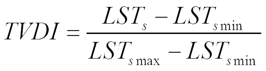
其中,湿边方程
LSTsmin = a * NDVI + b
干边方程
LSTsmax = c * NDVI + d
TVDI的值域为[0, 1]。
TVDI的值越大,表示土壤湿度越低,TVDI越小,表示土壤湿度越高。
干湿边拟合
在TVDI指数计算的过程中,需要拟合干边方程和湿边方程,其中还需要用户自己设置参数,是比较重要的计算步骤。拟合的关键是怎么找到有效的NDVI(相当于自变量X)和LST(相当于因变量Y)这两组相对应的数据,本文针对干湿边的拟合过程做一下详细的说明。
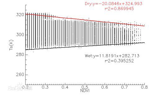
根据输入的NDVI和LST数据,以NDVI为横坐标,LST为纵坐标,可以得到NDVI-LST的散点图。根据NDVI-LST的散点图,就能得到每个NDVI值对应的LST的最大最小值,也就是我们要求的干边和湿边。具体步骤如下:
1)将NDVI等分为100份,分别为0~0.01,0.01~0.02,,,,,0.99~1.0(可根据具体情况进行修改);
2)在NDVI影像中查找每个范围内的NDVI值的索引,然后根据这些索引获取对应的LST数据的栅格值,求出每个范围内LST栅格值中的最大值和最小值;
3)将100份的LST栅格值分别求出最大值和最小值,就能得到NDVI-LST对应的干湿边的散点图,如下图所示;
4)设置NDVI的有效值范围(通常为0.2~0.8),选取有效范围内的数值进行线性拟合,得到干湿边方程。
Python实现TVDI计算
TVDI模型对干旱监测方面有重要的意义,但是目前的GIS和遥感软件中缺少计算TVDI的工具,要实现这个模型需要编程,做起来十分麻烦。有人利用ENVI/IDL来计算TVDI,开发出了TVDI计算补丁,但用起来很不灵活,有时还会出现未知错误,给用户造成很多困扰。
因此,本博客基于Python语言实现了TVDI的计算,详细代码如下:
导入必要的库
1 2 3 4 5 | import osimport mathimport numpyimport matplotlib.pyplot as pltfrom osgeo import gdal,osr |
首先,定义读取栅格数据的类函数,依赖GDAL python库。关于GDAL python库的安装,本文不做细讲,如需要可自行搜索学习。
1 2 3 4 5 6 7 8 9 10 11 12 13 14 15 16 17 18 19 20 21 22 23 24 25 26 27 28 29 30 31 32 33 34 35 36 37 38 39 40 41 42 43 44 | from osgeo import gdal,osrclass Raster: def __init__(self, nRows, nCols, data, noDataValue=None, geotransform=None, srs=None): self.nRows = nRows self.nCols = nCols self.data = data self.noDataValue = noDataValue self.geotrans = geotransform self.srs = srs self.dx = geotransform[1] self.xMin = geotransform[0] self.xMax = geotransform[0] + nCols * geotransform[1] self.yMax = geotransform[3] self.yMin = geotransform[3] + nRows * geotransform[5]def ReadRaster(rasterFile): ds = gdal.Open(rasterFile) band = ds.GetRasterBand(1) data = band.ReadAsArray() xsize = band.XSize ysize = band.YSize noDataValue = band.GetNoDataValue() geotrans = ds.GetGeoTransform() srs = osr.SpatialReference() srs.ImportFromWkt(ds.GetProjection()) # print srs.ExportToProj4() if noDataValue is None: noDataValue = -9999 return Raster(ysize, xsize, data, noDataValue, geotrans, srs)def WriteGTiffFile(filename, nRows, nCols, data, geotransform, srs, noDataValue, gdalType): format = "GTiff" driver = gdal.GetDriverByName(format) ds = driver.Create(filename, nCols, nRows, 1, gdalType) ds.SetGeoTransform(geotransform) ds.SetProjection(srs.ExportToWkt()) ds.GetRasterBand(1).SetNoDataValue(noDataValue) ds.GetRasterBand(1).WriteArray(data) ds = None |
编写主要的函数,包括干边、湿边提取拟合,以及计算TVDI
1 2 3 4 5 6 7 8 9 10 11 12 13 14 15 16 17 18 19 20 21 22 23 24 25 26 27 28 29 30 31 32 33 34 35 36 37 38 39 40 41 42 43 44 45 46 47 48 49 50 51 52 53 54 55 56 57 58 59 60 61 62 63 64 65 66 67 68 69 70 71 72 73 74 75 76 77 78 79 80 81 82 83 84 85 86 87 88 89 90 91 92 | def calTVDI(dir, in_ndvi_raster, in_lst_raster, ndvi_range, out_raster): ''' Calculate TVDI :return: ''' # 读取输入栅格数据信息 print("读取输入栅格数据信息...") raster_ndvi = ReadRaster(in_ndvi_raster) raster_lst = ReadRaster(in_lst_raster) ndvi = raster_ndvi.data lst = raster_lst.data nc = raster_ndvi.nCols nr = raster_ndvi.nRows geo = raster_ndvi.geotrans srs = raster_ndvi.srs ndv_ndvi = raster_ndvi.noDataValue ndv_lst = raster_lst.noDataValue abcd = edge(dir, ndvi, lst, nr, nc, ndv_ndvi, ndv_lst, ndvi_range) a = abcd[0][0] b = abcd[0][1] c = abcd[1][0] d = abcd[1][1] print("\t干边拟合方程:y = %.3fx + %.3f,r2 = %.3f" % (a, b, abcd[0][2] * abcd[0][2])) print("\t湿边拟合方程:y = %.3fx + %.3f,r2 = %.3f" % (c, d, abcd[1][2] * abcd[1][2])) tvdi = numpy.zeros((nr, nc)) for m in range(nr): for n in range(nc): if ndvi[m][n] != ndv_ndvi and lst[m][n] != ndv_lst: tvdi[m][n] = (lst[m][n] - (abcd[1][0] * ndvi[m][n] + abcd[1][1])) / ((abcd[0][0] * ndvi[m][n] + abcd[0][1]) - (abcd[1][0] * ndvi[m][n] + abcd[1][1])) else: tvdi[m][n] = ndv_ndvi # Save TVDI WriteGTiffFile(out_raster, nr, nc, tvdi, geo, srs, ndv_ndvi, gdal.GDT_Float32) print("计算完成\n\tSave as '%s'\n" % out_raster)def edge(dir, ndvi, lst, nr, nc, ndv_ndvi, ndv_lst, ndvi_range): ''' Get dry edge and wet edge :return: ''' print("干边、湿边拟合...") # 将NDVI按0.01间距分成100份,请注意NDVI值不要超过1.0 edgeArr = [[] for _ in range(100)] for i in range(nr): for j in range(nc): if ndvi[i][j] != ndv_ndvi and lst[i][j] != ndv_lst: if ndvi[i][j] > 0 and ndvi[i][j] < 1: k = "{:.2f}".format(ndvi[i][j]) k = int(k[2:]) # 取小数部分的前两位数字并转为整数 if lst[i][j] > -9999 and lst[i][j] < 9999: edgeArr[int(k)].append(lst[i][j]) # 排序,寻找干边湿边 eMax = [] ndviSort = [] eMin = [] for n in range(len(edgeArr)): edgeSort = numpy.sort(edgeArr[n]) if len(edgeSort) > 1: eMax.append(edgeSort[-1]) eMin.append(edgeSort[0]) ndviSort.append(float(n) / 100.) # 根据有效NDVI筛选数据 nMax = int(ndvi_range[1] * 100) nMin = int(ndvi_range[0] * 100) fiteMax = eMax[nMin:nMax] fiteMin = eMin[nMin:nMax] fitndviSort = ndviSort[nMin:nMax] fitMax = linefit(fitndviSort, fiteMax) fitMin = linefit(fitndviSort, fiteMin) # 保存拟合数据 outcsv = dir + os.sep + 'fit_data.csv' out = open(outcsv, 'w') out.write("NDVI,emax,emin\n") print("NDVI,emax,emin") for n in range(len(fitndviSort)): print("%.3f,%.3f,%.3f" % (fitndviSort[n], fiteMax[n], fiteMin[n])) out.write("%.3f,%.3f,%.3f\n" % (fitndviSort[n], fiteMax[n], fiteMin[n])) out.close() # 作图 outfig = dir + os.sep + 'fig.png' createPlot(fitndviSort, fiteMax, fiteMin, [fitMax, fitMin], outfig) return [fitMax, fitMin] |
用到的一些函数,如计算线性拟合参数、作图等
1 2 3 4 5 6 7 8 9 10 11 12 13 14 15 16 17 18 19 20 21 22 23 24 25 26 27 28 29 30 31 32 33 34 35 36 37 38 39 40 41 42 43 44 45 46 47 48 49 50 51 52 53 54 55 56 57 58 59 60 61 62 63 64 65 | def linefit(x, y): ''' Linear fitting :param x: :param y: :return: ''' N = float(len(x)) sx, sy, sxx, syy, sxy = 0, 0, 0, 0, 0 for i in range(0, int(N)): sx += x[i] sy += y[i] sxx += x[i] * x[i] syy += y[i] * y[i] sxy += x[i] * y[i] a = (sy * sx / N - sxy) / (sx * sx / N - sxx) b = (sy - a * sx) / N r = abs(sy * sx / N - sxy) / math.sqrt((sxx - sx * sx / N) * (syy - sy * sy / N)) return [a, b, r]def createPlot(ndvi, emax, emin, abcd, outfig): ''' Create plot :param ndvi: :param emax: :param emin: :param outfig: :return: ''' plt.rcParams['font.family'] = 'Times New Roman' fig, ax = plt.subplots(figsize=(8, 5)) plt.tick_params(labelsize=16) ylimit_min = numpy.min(emin) - 0.3 * numpy.average(emin) ylimit_max = numpy.max(emax) + 0.3 * numpy.average(emax) plt.ylim(ylimit_min, ylimit_max) plt.xlim(0, 1) cof = numpy.polyfit(ndvi, emax, 1) p = numpy.poly1d(cof) plt.plot(ndvi, p(ndvi), label='Dry edge fitting line', linewidth=1, c='#555555', linestyle='--') cof = numpy.polyfit(ndvi, emin, 1) p = numpy.poly1d(cof) plt.plot(ndvi, p(ndvi), label='Wet edge fitting line', linewidth=1, c='#555555', linestyle='--') plt.scatter(ndvi, emax, label='Dry edge', s=8, c='#FF4500') plt.scatter(ndvi, emin, label='Wet edge', s=8, c='#1E90FF') a = abcd[0][0] b = abcd[0][1] c = abcd[1][0] d = abcd[1][1] plt.text(0.05, ylimit_max / 2, "Dry edge: y = %.3fx + %.3f, r$^2$ = %.3f" % (a, b, abcd[0][2] * abcd[0][2]), color='#FF4500', fontsize=14) plt.text(0.05, ylimit_max / 3, "Wet edge: y = %.3fx + %.3f, r$^2$ = %.3f" % (c, d, abcd[1][2] * abcd[1][2]), color='#1E90FF', fontsize=14) ax.set_xlabel('NDVI', fontsize=16) ax.set_ylabel('LST ($^o$c)', fontsize=16) plt.legend(fontsize=16, loc='upper right', ncol=2) ax.grid(True, linestyle='--', alpha=0.3) fig.tight_layout() plt.savefig(outfig, dpi=300) print("\tSave as %s" % outfig) plt.show() |
应用方式
1 2 3 4 5 6 7 8 9 10 11 12 13 14 15 | if __name__ == "__main__": ## Define data path dataDir = r'<data path>' ## 输入文件 NDVIfile = dataDir + os.sep + 'NDVI.tif' LSTfile = dataDir + os.sep + 'LST.tif' ## 有效NDVI ndvi_range = [0.2, 0.8] ## 输出文件 outputfile = dataDir + os.sep + 'TVDI.tif' calTVDI(dataDir, NDVIfile, LSTfile, ndvi_range, outputfile) |
将上面几段代码粘贴在一个py文件中,设置文件路径,即可运行使用。
注意1:在计算干边、湿边过程中,会弹出matplotlib图形窗口,关闭后即可继续运行,图形保存在数据目录下。
在使用过程中遇到问题,可在下方评论处留言~
Fighting, GISer!
最新博文