
利用Matplotlib实现数据动态可视化
Data dynamic visualization by using Matplotlib
摘要
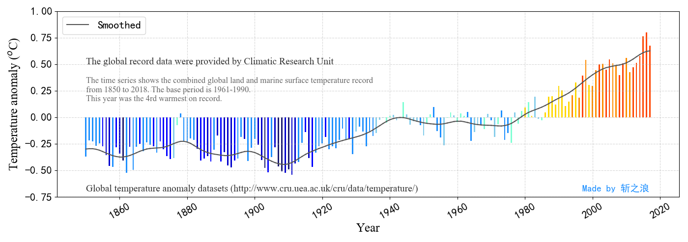
以1850-2018年150多年来全球平均气温距基准平均气温(1961-1990年)的变化数据为例,基于Matplotlib python库,绘制数据动态可视化图。
制作结果预览:
Matplotlib简单介绍
Matplotlib是Python中功能全面的绘图库。同时,它也可以与数学运算库NumPy、图形工具包PyQt和wxPython等多种python库一起使用,提供了一种有效的MatLab开源替代方案。
开发者使用Matplotlib,可以仅需要少量的代码,便可制作出专业、美观的直方图,条形图,功率谱,散点图等多种类型的图,是实现数据可视化的简单高效的工具。
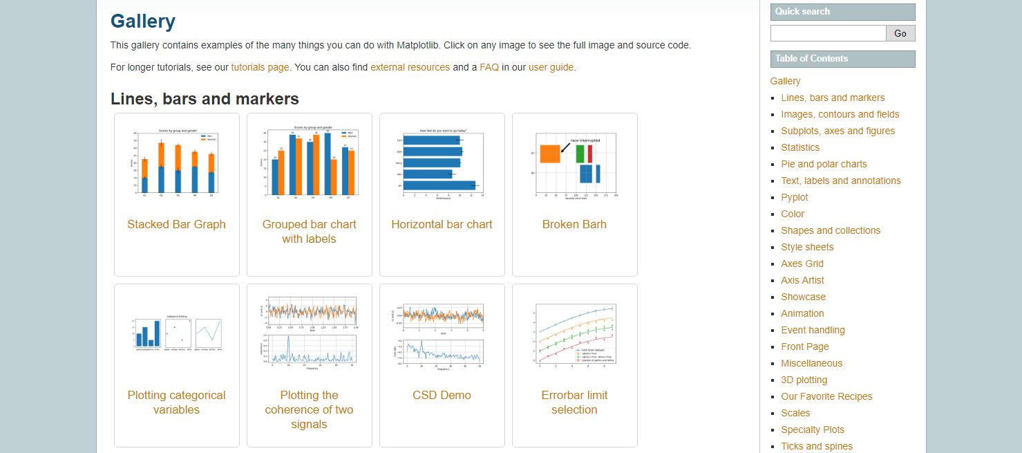
对于Matplotlib的安装、基本使用等,本文不再过多的介绍,在此附上官网链接,足够学习使用~
* 官方主页:https://matplotlib.org
* 官方示例:https://matplotlib.org/gallery/index.html
* 官方API:https://matplotlib.org/api/index.html
绘制动态图
一般情况下,利用Matplotlib绘制动态图时,通常选择使用Matplotlib的animation模块,但是该模块的函数使用比较繁琐,不易学习,开发不灵活。
因此,本文介绍一种相对比较简单的办法,使用动态绘图和暂停功能来实现,具体看代码。
1 2 3 4 5 6 7 8 9 10 11 12 13 14 15 16 17 18 19 20 21 22 23 24 25 26 27 28 29 30 31 32 33 34 35 36 37 38 39 40 41 42 43 44 45 46 47 48 49 50 51 52 53 54 55 56 57 58 59 60 61 62 63 64 65 66 67 68 69 70 71 72 73 74 75 | # -*- coding: utf-8 -*-import numpyimport matplotlib.pyplot as pltimport matplotlib.dates as mdate# 配置参数plt.rcParams['font.family'] = 'Times New Roman' # 设置字体plt.rcParams['axes.unicode_minus'] = False # 用来正常显示负号# 设置字体大小fs_label = 18fs_ticks = 16fs_legend = 16fs_text = 16def Plot(x, y1, y2): ''' Create plot :param x: :param y1: :param y2: :return: ''' fig, ax = plt.subplots(figsize=(14, 5)) # 创建窗口和子图 plt.tick_params(labelsize=fs_ticks) # 设置刻度字体 # 设置时间轴格式 fig.autofmt_xdate(rotation=30, ha='center') dateFmt = mdate.DateFormatter('%Y') ax.xaxis.set_major_formatter(dateFmt) years = numpy.arange(int(x[0]), int(x[-1]) + 1) yearsDate = GetDateArr(years) # 获取年份列表 xs = [yearsDate[0], yearsDate[0]] ys = [y1[0], y1[0]] ys2 = [y2[0], y2[0]] # 添加text plt.text(yearsDate[-22], -0.7, 'Made by GaoHR', fontsize=fs_text-2, color='#1E90FF') plt.text(yearsDate[0], -0.7, 'Global temperature anomaly datasets (http://www.cru.uea.ac.uk/cru/data/temperature/)', fontsize=fs_text-2, fontfamily='Times New Roman', color='#333333') plt.text(yearsDate[0], 0.5, 'The global record data were provided by Climatic Research Unit', fontsize=fs_text-2, fontfamily='Times New Roman', color='#333333') plt.text(yearsDate[0], 0.15, 'The time series shows the combined global land and marine surface temperature record\n' 'from 1850 to 2018. The base period is 1961-1990.\n' 'This year was the 4rd warmest on record.', fontsize=fs_text-4, fontfamily='Times New Roman', color='#666666') # 设置x、y轴范围 # plt.xlim(x_min, x_max) plt.ylim(-0.75, 1) # 设置标签、添加刻度标线 ax.set_xlabel('Year', fontsize=fs_label, fontfamily='Times New Roman') ax.set_ylabel('Temperature anomaly ($^o$C)', fontsize=fs_label, fontfamily='Times New Roman') plt.grid(True, linestyle='--', alpha=0.5) # 动态读取数据,绘制图形 for i in range(years[0], years[-1]): # 更新x, y1, y2 xs[0] = xs[1] ys[0] = ys[1] ys2[0] = ys2[1] xs[1] = yearsDate[i - int(x[0])] ys[1] = y1[i - int(x[0])] ys2[1] = y2[i - int(x[0])] ax.bar(xs, ys, width=150, color=getColor(y1[i - int(x[0])])) # 绘制条状图 ax.plot(xs, ys2, color='#555555') # 绘制曲线图 plt.legend(['Smoothed'], loc='upper left', fontsize=fs_legend) # 添加图例 plt.pause(0.1) # 设置时间间隔 plt.tight_layout() plt.show() |
还有用到的一些函数:读取Excel表格函数ReadDatafromExcel,不同值显示不同的颜色getColor等
1 2 3 4 5 6 7 8 9 10 11 12 13 14 15 16 17 18 19 20 21 22 23 24 25 26 27 28 29 30 31 32 33 34 35 36 37 38 39 40 41 42 43 44 45 46 47 48 49 50 51 52 53 54 55 56 57 58 | def ReadDatafromExcel(xlsfile, sheet_name, ytype, yindex, t_index=[]): ''' Read data from excel :param xlsfile: :param sheet_name: :param ytype: :param yindex: :param t_index: :return: 2-D array ''' bk = xlrd.open_workbook(xlsfile) y = [] for sh in bk.sheets(): # print len(sh.col_values(0)) # print "Sheet:", sh.name if sh.name == sheet_name: # y = numpy.zeros((len(ytype), days_num)) for j in range(len(ytype)): k = [] # col_len = len(filter(lambda x: x != "", sh.col_values(j))) # 获取列的长度 row_len = sh.nrows if j not in t_index: for i in range(row_len - 1): k.append(sh.cell(i + 1, yindex[j]).value) y.append(k) else: # 如果是时间字段,则读取为 datetime 类型 for i in range(row_len - 1): k.append(xlrd.xldate.xldate_as_datetime(sh.cell(i + 1, yindex[j]).value, bk.datemode)) y.append(k) return ydef getColor(t): ''' Get color based on t :return: ''' if t < -0.5: return "#191970" elif -0.5 < t < -0.4: return "#0000CD" elif -0.4 < t < -0.3: return "#0000FF" elif -0.3 < t < -0.1: return "#1E90FF" elif -0.1 < t < 0: return "#87CEEB" elif 0 < t < 0.1: return "#7FFFD4" elif 0.1 < t < 0.3: return "#FFD700" elif 0.3 < t < 0.4: return "#FF8C00" elif 0.4 < t < 0.5: return "#FF8C00" else: return "#FF4500" |
主函数
1 2 3 4 5 6 7 8 9 10 11 | if __name__ == "__main__": xlsfile = r"<Excel文件路径>" sheet_name = "Sheet1" ytype = ["x", " y1", "y2"] yindex = [0, 1, 2] data = ReadDatafromExcel(xlsfile, sheet_name, ytype, yindex) x = data[0] y1 = data[1] y2 = data[2] Plot(x, y1, y2) |
补充
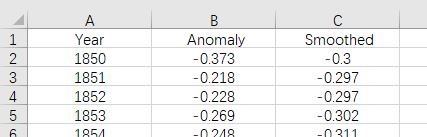
需要注意的是,本文代码读取的Excel表格格式如下图所示。
数据可以从Global temperature anomaly datasets网站上获取。
附绘制的数据静态图
Fighting, GISer!
最新博文